In order to produce reliable computational fluid dynamics (CFD) results, the mesh resolution can have a severe impact on both, qualitative and quantitative simulation results. Judging a mesh appropriate for the case one wants to analyze depends on many factors, such as operating point and required accuracy of the results.
In the field of rotary positive displacement (PD) machines, especially leakage flows caused by clearances between rotors as well as between rotors itself and housing are of great interest, because they can affect the overall machine efficiency. The clearances are very small compared to the global machine scale and the numerical mesh has to resolve those clearances, when considering them to be part of the numerical model.
In the following blog we will present data from three different cases where the correct mesh resolution is inevitable. Read through the text, have a look at the data, and be stunned by the fact that a coarse mesh resolution will give you poor and in the worst case unreliable results.
Test Case 1: 2D and 3D Lobe Pump (incompressible)
We performed a 2D test case including only radial clearances and a 3D test case with radial and axial clearances of a lobe pump with water at 1000 rpm and a pressure ratio of 10:1. Both cases were carried out on a very coarse grid as well as on a fairly fine mesh to elaborate the influence of the mesh on the results. For the 2D test case, a mesh without inflation layers towards the walls while maintaining a fine resolution everywhere else was added to the comparison.
 and fine mesh (right)")
, fine grid without inflation layer (center) and the fine grid with inflation layer (bottom) towards the rotor walls")
Regarding the flow conditions within the lobe pump, all grids show qualitative similar results as you can see in the velocity plots on the left hand side. However, they differ when quantifying the velocity field. This is observed for the 2D as well as for the 3D case. Examining the 2D results, differences in the velocity maxima are found within the working chambers as well as downstream (pressure side). This is due to the coarse mesh, while the fine mesh and the fine mesh without wall refinement provide almost equal results given the used resolution and element height at the rotor wall. Therefore, we will examine this issue further in a third test case.
Analyzing this on the basis of the 3D simulation, the global maximum on the cross-section plane is located within the interlobe clearance for the fine mesh, whereas for the coarse grid case, it is found in the radial gap between lobe and housing. Both matches the expectation, finding the highest velocities in clearances. So it is rather an order of magnitude than the location that attracts the attention when comparing the velocity distribution for the fine and the coarse mesh. Here the maximum velocity derived on the fine mesh is twice as high as the maximum velocity on the coarse grid.
 and the fine grid (right)")
 and fine grid (right)")
The figure on the left illustrates flow regimes within the clearances between rotor and housing as well as the clearance between the two rotors. Here again, the fine mesh leads to significant higher velocity within the small gap between the rotors, surpassing the coarse mesh results by about 53%. Moreover there is a sharper distinction of the leakage flow within the radial gaps.
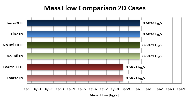
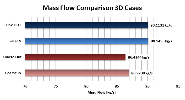
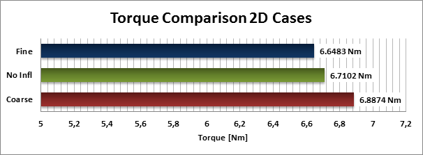
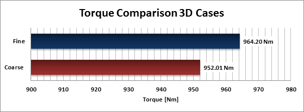
The charts in the gallery on the right hand side show integral characteristics of the pump such as mass flow and torque which can be analyzed within a CFD simulation. For our case both values are averaged over one complete rotor revolution. Again we can see notable differences between the results using the coarse mesh resolution and the fine meshes with and without refinement in the boundary layer.
Test Case 2: 3D Screw Compressor (compressible)
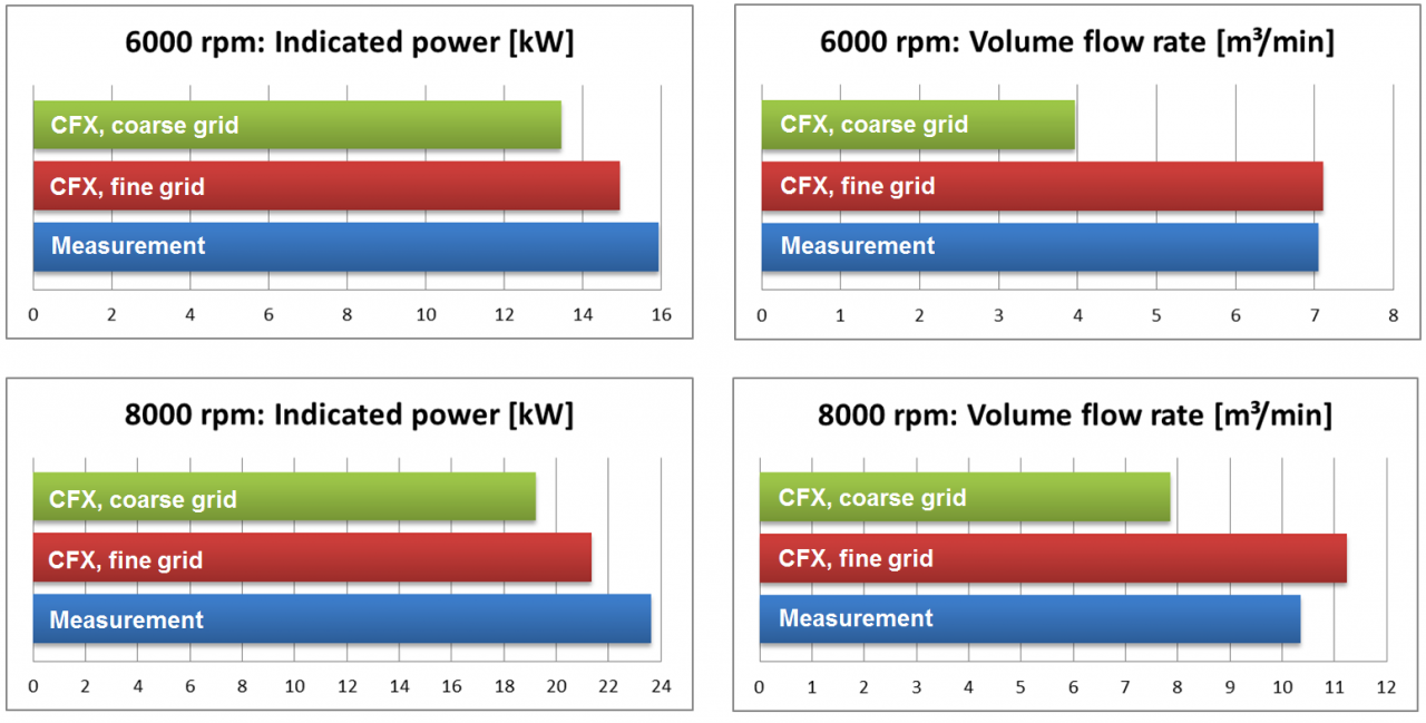
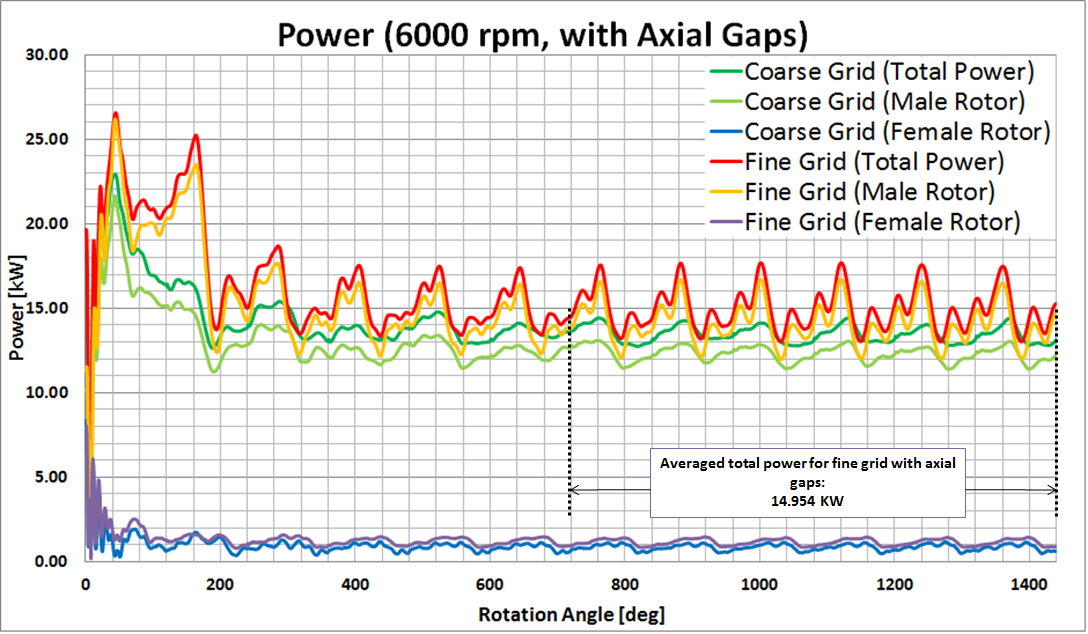
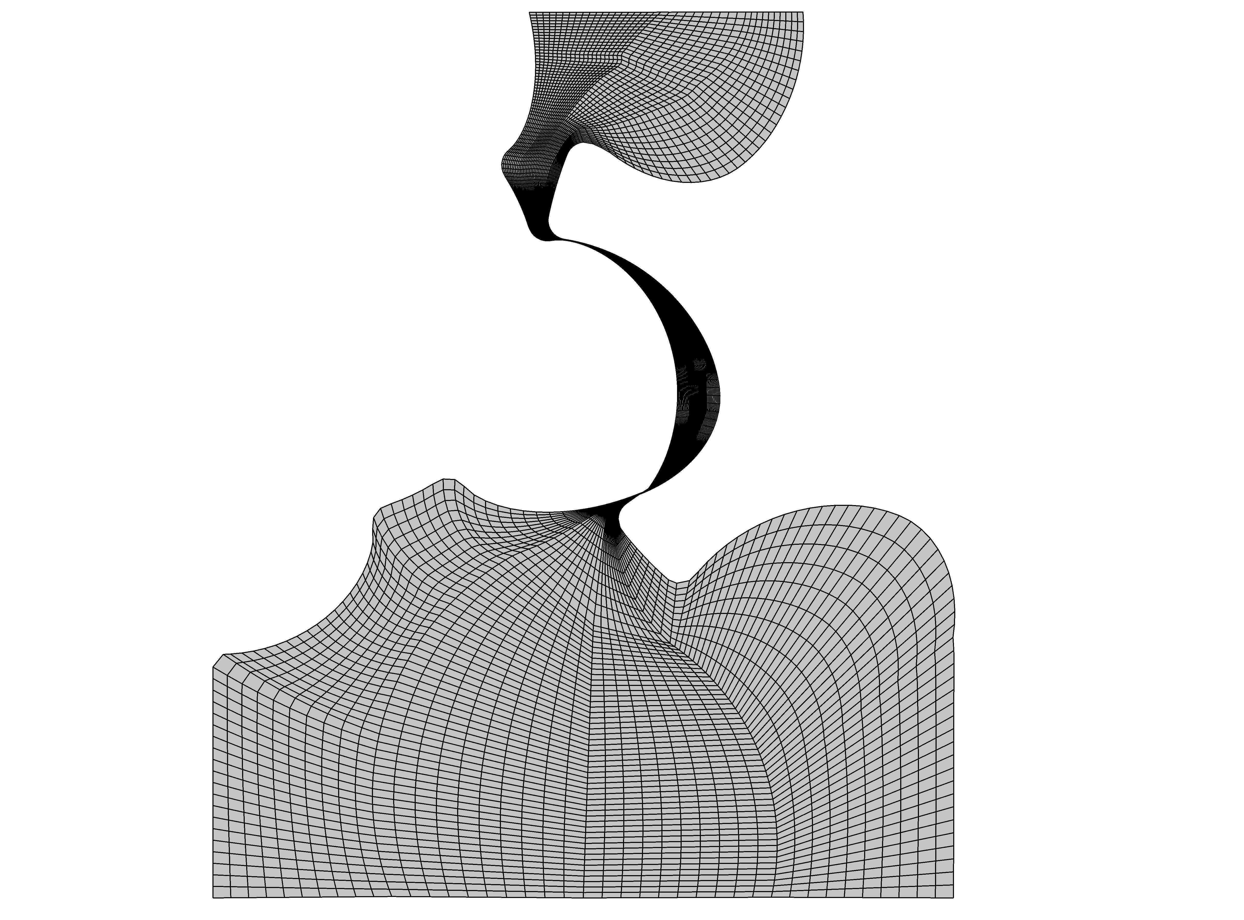
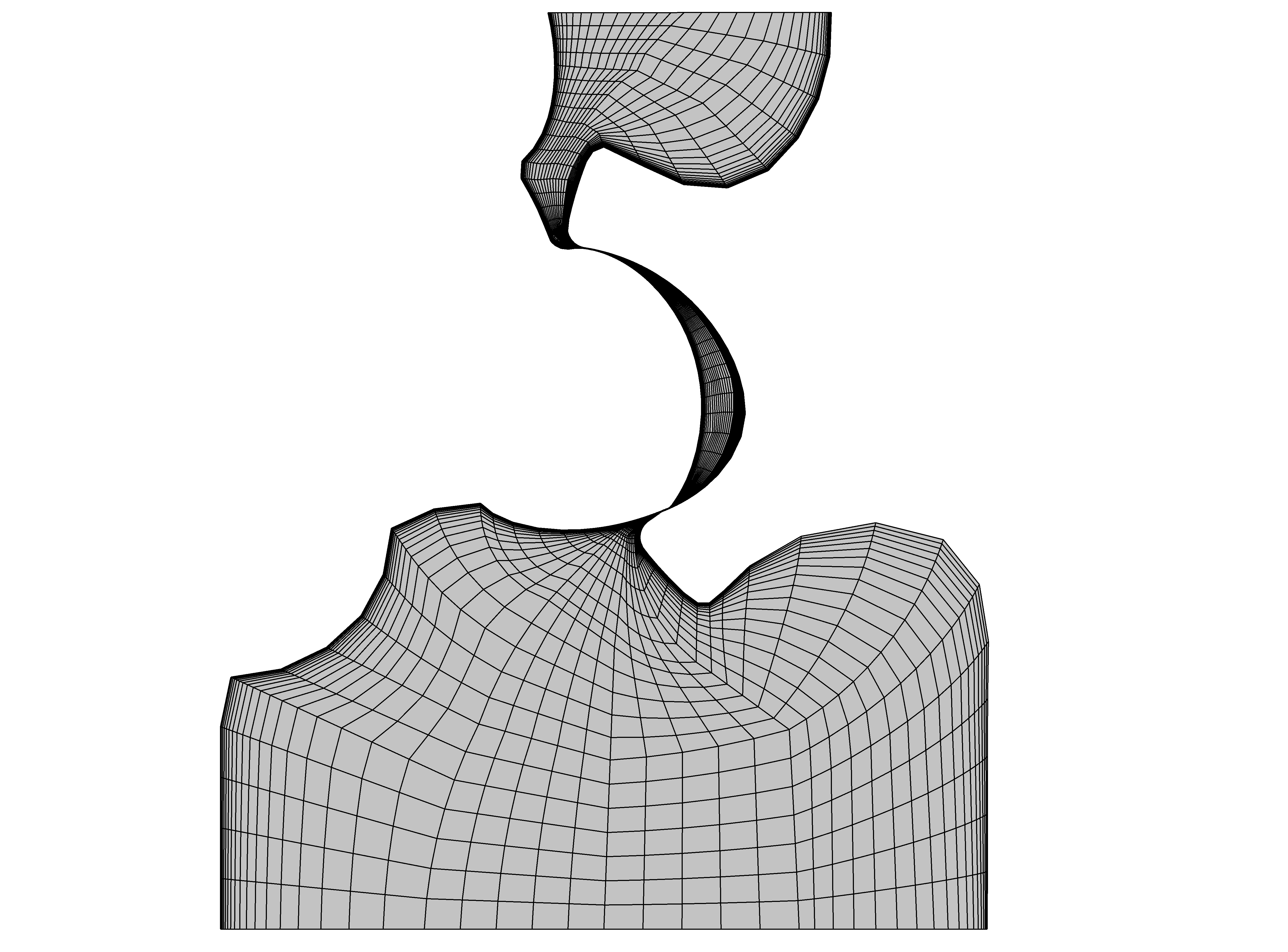
The second test case for this study incorporates results of a dry running screw compressor, which were also presented by us during the short course session at the International Conference on Compressors and their Systems 2015 in London. For this analysis two operation points were simulated and compared with measurements, while here the influence of the mesh resolution is exemplified. The picture on the right hand side shows the numerical meshes used in this case.
Once more, fine mesh and coarse mesh results are compared to each other. Taking a look at the velocity field over time, results show more distinct maxima for the fine mesh case, which was also seen in our first test case aforementioned. A video of the transient velocity fields for the fine and the coarse mesh is shown below this paragraph.
 and the fine case (bottom)")
If you are interested in more details of this screw compressor test case you can download a copy of slides of the short course on screw compressor CFD simulation given by Dr. Andreas Spille-Kohoff at the ICCS 2015 in London.
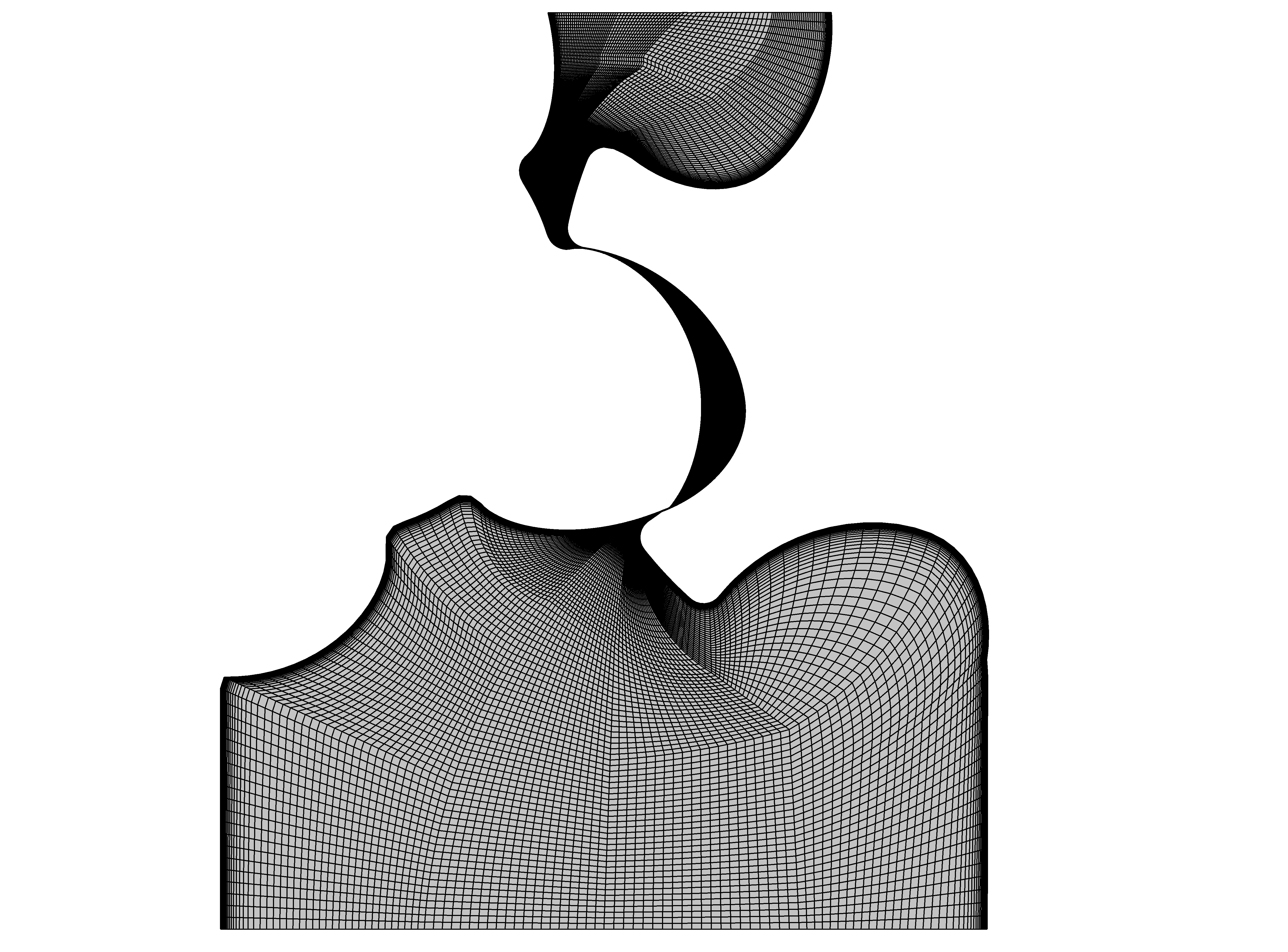
Test Case 3: Steady State Flow through an Interlobe Clearance of a SRM Rotor Profile (Compressible)
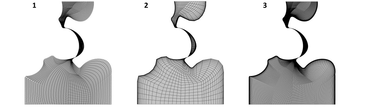
The third test case is based on a 2D steady-state simulation of compressible air flow through the interlobe clearance of a SRM rotor profile with an operating pressure ratio of 3:1. Again the simulations were carried out on different meshes in order to determine the mass flow corresponding to the spatial discretization. Grids (1) and (2) have a similar overall number of elements, whereas grid (2) incorporates wall refinements and grid (1) has a uniform element distribution. Grid (3) is a very fine mesh for this case setup and will be used as a reference. All numerical grids are shown in the slide show on the right hand side.

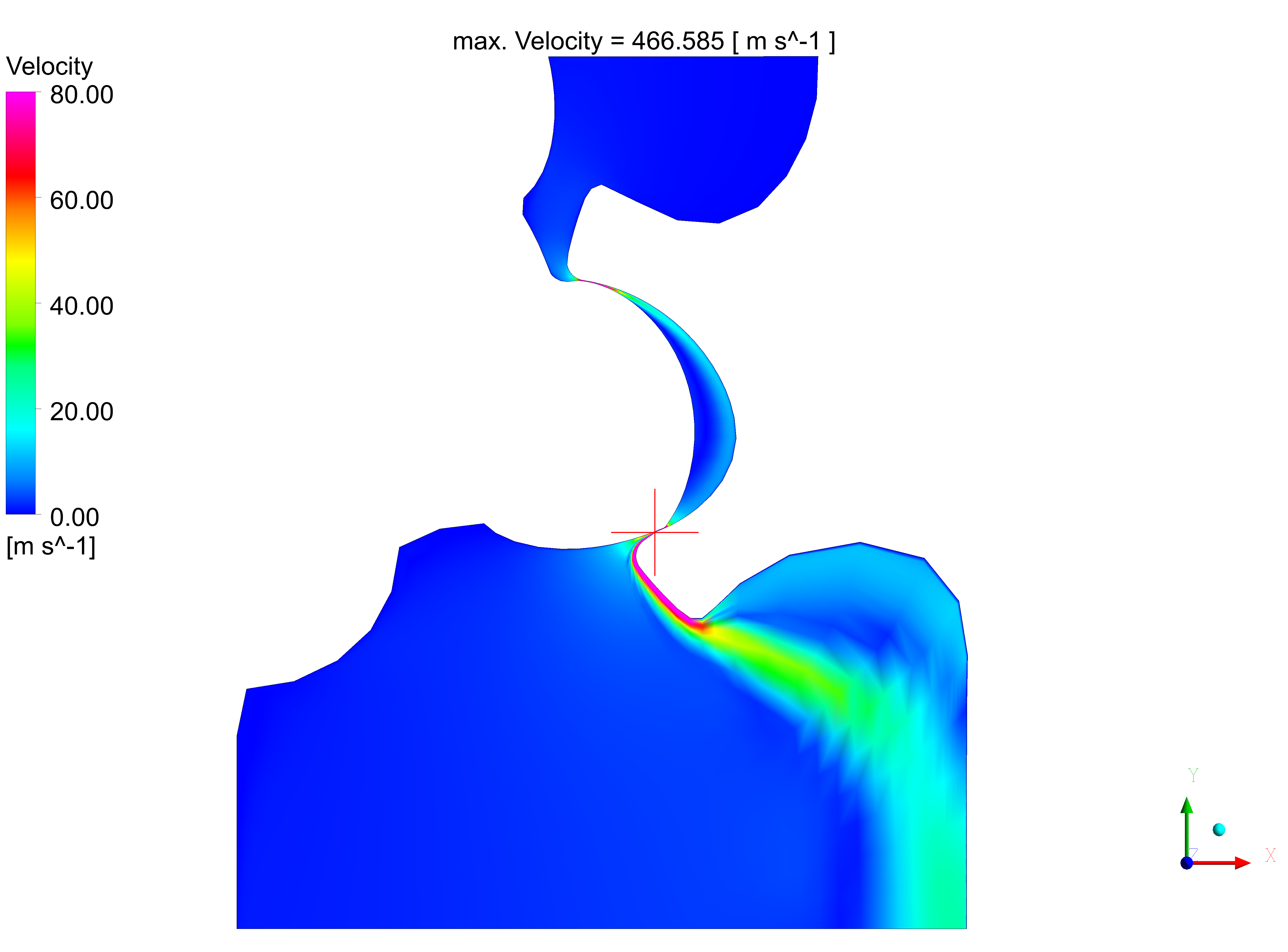
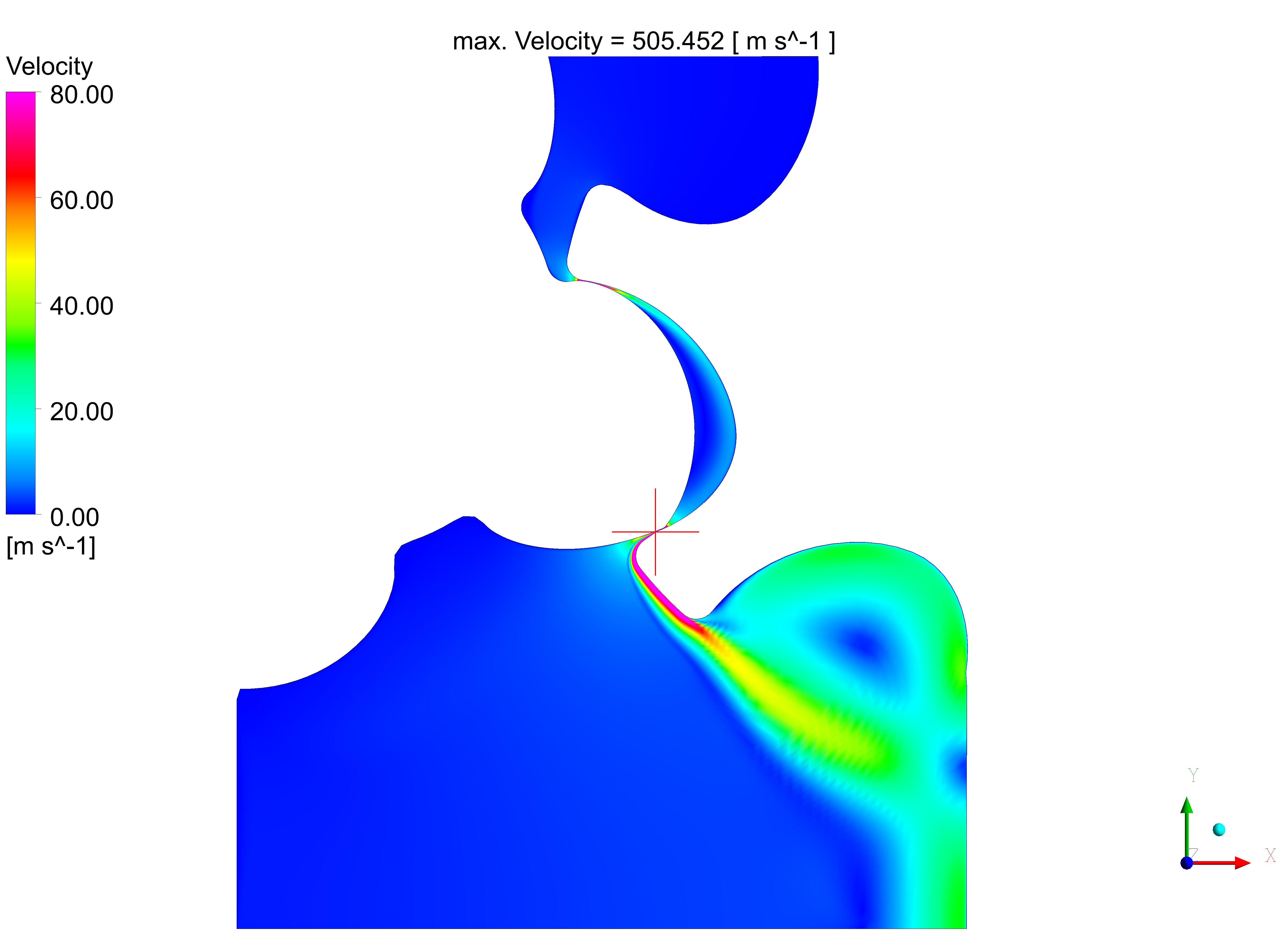
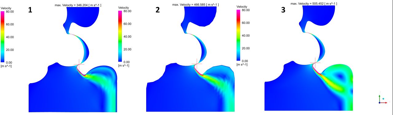
The velocity flow field plots on the left show significant deviations from the reference solution on the coarse grids. Although the location of the maximum velocity matches for all simulations, the solution on grid (1) yields the lowest maximum velocity of all grids, while grid (2) already reaches 92% of the reference value. Likewise the velocity along the jet streamlines is underestimated by grids (1) and (2). Moreover the jet characteristics on grid (1) differ from the reference solution especially in the intermesh zone between the lobes. Concerning grid (2) the jet alignment both in the intermeshing zone and downstream of the flow separation show a fairly good agreement with the reference solution. However, the fine grid grants a more detailed insight into the flow field for the recirculation zone and boundary layers.
 and without (red bar) inflation layer towards the walls and the fine grid (blue bar)")
Conclusion
As shown by our test case results, mesh resolution affects the simulation results significantly. While this is an inevitable fact due to spatial discretization, the relevance for daily CFD engineering has to be determined.
As shown in the first test case for the simple 2D simulation of the lobe pump, the differences between coarse grid and fine grid results are fairly moderate, when considering integral flow values. Deviation between the two results is within a single-digit percentage range. The difference increases clearly, if local resolved maxima are taken into account, diverging up to 100%.
The same observations hold up for the second and the third test case, where in the case of the screw compressor, even the integral value of the volume flow derived on the coarse grid was off by 75% compared to the fine grid results (6000 rpm).
The simulation of the 2D SRM rotor profile in the third test case yields similar results. Both local resolved maxima and integral flow values differ significantly for different mesh resolutions. Furthermore, the influence of the adequate resolution of the boundary layer can be observed in this setup.
An evaluation of these findings is a tough task for the engineer, as experimental data are often not available or limited to integral values. The coarse grids that were used in our test cases cannot be judged to produce poor results in general. Although, considered to be rather at the bottom end of how coarse the mesh can be without losing reasonable geometry representation, they are in fact able to provide results that are very close to fine grid results. Especially regarding the much shorter computation time on the coarse grids, this can be a true advantage in the early stages of the development process.
As optimization of today’s available PD machines is of interest, proper representation of clearances and thus, a more accurate approximation of the adjacent rotor and housing geometry is very important. It is concluded that very coarse meshes have restrictions in fulfilling this purpose and as a consequence, leakage flows are not properly resolved. The complex 3D case of the screw compressor indicates that this can affect the pressure build up, leading to lower volume flow at the pressure side eventually. However, this assumption alone does not accommodate for an exhaustive analysis of the complex flow physics within this machine type and the interaction between those physics, discretized on the computational grid in space and time.
In summary, generalizations should be made cautiously. It is evident that requirements on both, CFD grids and numerical models rise along with the desired insight and accuracy. While numerics are deeply integrated in the CFD solver the engineer uses, the ability to adapt mesh resolution to the current task without sacrificing mesh quality certainly enhances the CFD workflow and results. It enables short time simulations as well as a complex analysis incorporating all physical models available in the CFD solver.
